What is linear regression?

• Models the relationship between a continuous dependent variable \(y\) and one or more independent variables \(x\).
• Finds a straight-line fit between variables
• Why?
  • Measure the strength of a relationship
  • Understand the nature of a relationship
  • Predict \(y\) for new values of \(x\)

Simple linear regression

• Models the relationship between a single independent variable \(x\) and a dependent variable \(y\).
• Independent variable may also be called an explanatory or predictor variable.
• Dependent variable may be called the response.

Example

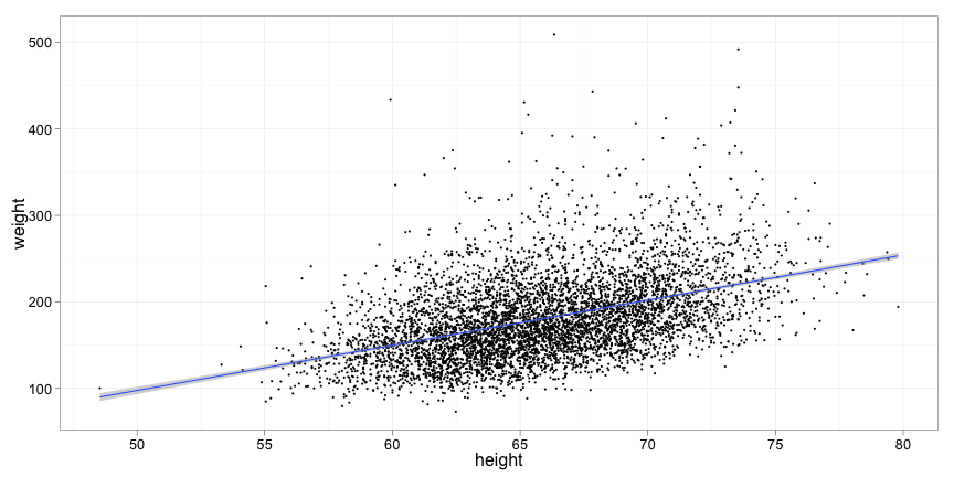
What is the relationship between height and weight?

library(ggplot2)
data = read.csv("CDC_data.csv")
p = qplot(height, weight, data = data, size = I(1))
p + stat_smooth(method = "lm")

Source: CDC National Health and Nutrition Examination Survey 2009-2010

The linear regression model

Simple linear regression uses the model \[y_i = \beta_0 + \beta_1 x_i + \epsilon_i\]

• The \(y_i\) are the dependent variables
• The \(x_i\) are the independent variables
• \(\beta_0\) is the intercept of the line and \(\beta_1\) is the slope
• You may recognize this from linear algebra as the formula for a line
• \(\epsilon_i\) is the error term for each \(y_i\)—the difference between the actual \(y_i\) and the predicted value
• The error terms are assumed to be normal, independent and identically distributed

Finding the best line

• Find the values for \(\beta_0\) and \(\beta_1\) that minimize the sum of squared errors \(\sum{\epsilon_i^2}\). This is the least squares fit.

• In R this is done with the stats::lm() function.

• lm() uses a formula interface to specify the dependent and independent variables.

• The formula y ~ x means “y is modeled by x.”

• In the example we want to model weight as a function of height so the formula is

  weight ~ height

Example (cont)

model = lm(weight ~ height, data)
summary(model)

# 
# Call:
# lm(formula = weight ~ height, data = data)
# 
# Residuals:
#    Min     1Q Median     3Q    Max 
#  -92.7  -28.9   -6.3   21.4  325.7 
# 
# Coefficients:
#             Estimate Std. Error t value Pr(>|t|)    
# (Intercept) -163.233      8.882   -18.4   <2e-16 ***
# height         5.218      0.135    38.8   <2e-16 ***
# ---
# Signif. codes:  0 '***' 0.001 '**' 0.01 '*' 0.05 '.' 0.1 ' ' 1 
# 
# Residual standard error: 42.3 on 5992 degrees of freedom
# Multiple R-squared:  0.2, Adjusted R-squared:  0.2 
# F-statistic: 1.5e+03 on 1 and 5992 DF,  p-value: <2e-16 
# 

What?

• The formula used to create the model:

  # Call:
  # lm(formula = weight ~ height, data = data)

• Residuals are the error terms \(\epsilon_i\)—smaller is better:

  # Residuals:
  #    Min     1Q Median     3Q    Max 
  #  -92.7  -28.9   -6.3   21.4  325.7 

• The coefficient estimates are the model parameters. (Intercept) is \(\beta_0\), the intercept of the line on the y-axis. height is \(\beta_1\), the slope of the line.

  # Coefficients:
  #             Estimate   
  # (Intercept) -163.233
  # height         5.218

• In this model, an additional inch of height translates to 5.2 pounds weight.

Model statistics

The rest of the output is useful for evaluating the model. It includes

• standard error, t-statistic and p-value for each coefficient

  # Coefficients:
  #             Estimate Std. Error t value Pr(>|t|)    
  # (Intercept) -163.233      8.882   -18.4   <2e-16 ***
  # height         5.218      0.135    38.8   <2e-16 ***

• \(R^2\) value and F-statistic

  # Residual standard error: 42.3 on 5992 degrees of freedom
  #   (65 observations deleted due to missingness)
  # Multiple R-squared:  0.2, Adjusted R-squared:  0.2 
  # F-statistic: 1.5e+03 on 1 and 5992 DF,  p-value: <2e-16 

Confidence intervals

Confidence intervals on the model coefficients are another way to evaluate the model. The stats::confint() function computes confidence intervals for model coefficients.

confint(model)

#                2.5 %   97.5 %
# (Intercept) -180.645 -145.820
# height         4.954    5.482

Graphical evaluation of the model

Not all data is well represented by a linear model.

• Non-linear data, e.g. quadratic, exponential
• Error terms are not normal and independent
  • Non-normal distribution
  • Depend on prediction
  • Non-equal variances
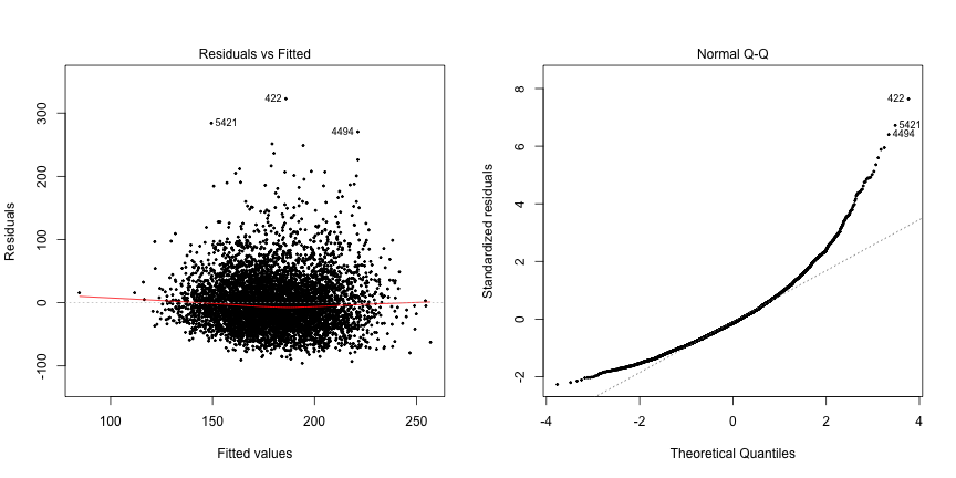
• plot(model) creates diagnostic plots

Diagnostic plots

op <- par(mfrow = c(1, 2))
plot(model, which = c(1, 2), pch = 20, cex = 0.5)

Hmmm…

The diagnostic plots indicate that the errors are not normally distributed. They seem to be skewed toward the right, i.e. the tail is longer on the right. This is visible in the original plot as well.

In the real world, you might try transforming the data to get a better fit.

Predictions

The stats::predict() function is used to predict the \(y\) values for new values of \(x\).

Values for the independent variable are passed in a data frame column with the same name as the original data.

new_x = data.frame(height = c(60, 65, 70))
predict(model, new_x)

#     1     2     3 
# 149.9 176.0 202.1 

Predictions may include confidence intervals:

predict(model, new_x, interval = "prediction")

#     fit   lwr   upr
# 1 149.9  66.9 232.8
# 2 176.0  93.0 258.9
# 3 202.1 119.1 285.0

Multiple regression

Multiple regression models the dependent variable as a linear combination of multiple independent variables.

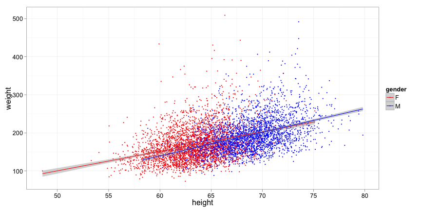
• For example, how does gender affect the relationship between height and weight?

• The simplest case has no interactions between the independent variables: \[y_i = \beta_0 + \beta_1 x_{1i} + \beta_2 x_{2i} + ... + \beta_n x_{ni} + \epsilon_i\]

• For height, weight and gender this becomes \[weight_i = \beta_0 + \beta_1 height_i + \beta_2 gender_i + \epsilon_i\]

• The R formula is similar to the model: weight ~ height + gender

Example (cont)

model <- lm(weight ~ height + gender, data)
summary(model)

# 
# Call:
# lm(formula = weight ~ height + gender, data = data)
# 
# Residuals:
#    Min     1Q Median     3Q    Max 
#  -95.9  -28.9   -6.0   21.5  322.7 
# 
# Coefficients:
#             Estimate Std. Error t value Pr(>|t|)    
# (Intercept) -191.437     11.528  -16.61  < 2e-16 ***
# height         5.688      0.182   31.25  < 2e-16 ***
# genderM       -5.665      1.479   -3.83  0.00013 ***
# ---
# Signif. codes:  0 '***' 0.001 '**' 0.01 '*' 0.05 '.' 0.1 ' ' 1 
# 
# Residual standard error: 42.3 on 5991 degrees of freedom
# Multiple R-squared: 0.202,    Adjusted R-squared: 0.202 
# F-statistic:  760 on 2 and 5991 DF,  p-value: <2e-16 
# 

What?

• The (Intercept) and height coefficients have the same meaning as before. The genderM coefficient models the difference in weight for a male and female of the same height. Surprisingly, in this model, males weigh on average 5.6 pounds less than females of the same height.

  # Coefficients:
  #             Estimate Std. Error t value Pr(>|t|)    
  # (Intercept) -191.437     11.528  -16.61  < 2e-16 ***
  # height         5.688      0.182   31.25  < 2e-16 ***
  # genderM       -5.665      1.479   -3.83  0.00013 ***

• All three coefficients are significant—they contribute to the model.

• The model statistics are similar before:

  # Residual standard error: 42.3 on 5991 degrees of freedom
  #   (65 observations deleted due to missingness)
  # Multiple R-squared: 0.202,    Adjusted R-squared: 0.202 
  # F-statistic:  760 on 2 and 5991 DF,  p-value: <2e-16 

Diagnostics again

op <- par(mfrow = c(1, 2))
plot(model, which = c(1, 2), pch = 20, cex = 0.5)

Interaction terms (briefly)

Does the slope of the relationship between height and weight depend on gender? This is an interaction. The model for this is

\[weight_i = \beta_0 + \beta_1 height_i + \beta_2 gender_i + \beta_3 height_i weight_i + \epsilon_i\]

The R formula uses * instead of +: weight ~ height * gender

Example (cont)

model <- lm(weight ~ height * gender, data)
summary(model)

# 
# Call:
# lm(formula = weight ~ height * gender, data = data)
# 
# Residuals:
#    Min     1Q Median     3Q    Max 
#  -95.4  -29.0   -5.9   21.6  324.5 
# 
# Coefficients:
#                Estimate Std. Error t value Pr(>|t|)    
# (Intercept)    -155.139     16.619   -9.34   <2e-16 ***
# height            5.114      0.263   19.47   <2e-16 ***
# genderM         -78.289     24.010   -3.26   0.0011 ** 
# height:genderM    1.103      0.364    3.03   0.0025 ** 
# ---
# Signif. codes:  0 '***' 0.001 '**' 0.01 '*' 0.05 '.' 0.1 ' ' 1 
# 
# Residual standard error: 42.2 on 5990 degrees of freedom
# Multiple R-squared: 0.204,    Adjusted R-squared: 0.203 
# F-statistic:  510 on 3 and 5990 DF,  p-value: <2e-16 
# 

```
# Coefficients:
#                Estimate Std. Error t value Pr(>|t|)    
# (Intercept)    -155.139     16.619   -9.34   <2e-16 ***
# height            5.114      0.263   19.47   <2e-16 ***
# genderM         -78.289     24.010   -3.26   0.0011 ** 
# height:genderM    1.103      0.364    3.03   0.0025 ** 
```

• (Intercept) is the intercept for the line for females
• height is the slope for females - on average, females weigh 5.1 pounds more for every inch of height
• genderM is the difference in intercept for males
• height:genderM is the difference in slope for males - on average, males weigh 5.1+1.1 pounds more for every inch of height

ggplot rocks!

p = qplot(height, weight, data = data, color = gender, size = I(1))
p + stat_smooth(method = lm) + scale_color_manual(values = c("red", 
    "blue"))